Analysis of Nanopore HEK293 with JACUSA2helper

This vignette requires the latest version of JACUSA2helper - please update*

In the following, the workflow for use case 3 from Piechotta et al. (2021) is presented. Data for use cases 1-3 can be downloaded to repeat the analysis.

The following packages need to be loaded:

library(JACUSA2helper)
library(GenomicRanges)
library(BSgenome)
library(GenomeInfoDb)
library(plyranges)
library(magrittr)
library(dplyr)
library(ggplot2)
library(pROC)
library(VennDiagram)
library(NMF)

Non-negative Matrix Factorization

Here, we briefly introduce Non-negative Matrix Factorization (NMF). This section uses the notation from NMF vignette.

Non-negative Matrix Factorization tries to find an approximation of: \[X \approx W H,\] where:

$X$ is a non-negative $n \times p$ matrix,
$W$ is a non-negative $n \times r$ matrix (basis matrix), and
$H$ is a non-negative $r \times p$ matrix (coefficient matrix).

$r$ is called the factorization rank.

Check NMF vignette for details on optimization and algorithms.

In the following, we will explain how to convert JACUSA2 output to an appropriate matrix $X$ and perform NMF.

General workflow

Use read_result to read JACUSA2 output and filter the data set.

To repeat the Nanopore analysis from Piechotta et al. (2021), download the following data:

WT vs. KO and
WT100 vs. WT0.

Depending on your bandwidth the Download might take some time. Download the data, start R and change into the directory where you have saved the files from zenodo. Make sure, you have approx. 20GB of main memory available.

Pre-processing

We start to organize the data:

# files to read
files <- c(
  "WT_vs_KO_call2_result.out.gz",
  "WT100_vs_WT0_call2_result.out.gz"
)

# descriptions corresponding to files 
meta_conds = c(
  "WT_vs_KO",
  "WT100_vs_WT0"
)

meta_conds is used as a concise description of each file to distinguish the JACUSA2 outputs.

The pre-processing workflow for one file can be summarized into the following steps:

Read: Read JACUSA2 output.
Filter: Employ coverage and other filters to remove not interesting sites.
Add meta condition: Add concise description of each file.
Reduce: Select relevant data column.

We explain the pre-processing workflow for one file and generalize to arbitrary number of files (here two).

Read

The underlying function of read_result is data.table::fread - check the respective help page for details on additional options. Depending on your machine increase nThreads to use more threads to parse a file.

The “info” field contains meta information for sites, such as detailed INDEL statistics. To save memory, we manually unpack the “info” field and select the following keys:

insertion_score and
deletion_score.

We will use these score values during model training.

i <- 1 # WT_vs_KO
print(files[i])
#> [1] "/home/michael/TODO/JACUSA2helper/WT_vs_KO_call2_result.out.gz"
print(meta_conds[i])
#> [1] "WT_vs_KO"

wt_vs_ko_res <- read_result(files[i], nThread = 2, unpack = c("insertion_score", "deletion_score"))

Filter

The JACUSA2 output files from Zenodo have been already filtered to retain sites with coverage $> 4$ in all BAM files.

We use the following filter:

retain sites on chromosome 1-22, MT, and X.

print(paste0("Sites BEFORE filtering: ", length(wt_vs_ko_res)))
#> [1] "Sites BEFORE filtering: 8891484"

# reduce set of known sequences
seqlevels(wt_vs_ko_res, pruning.mode = "coarse") <- c(1:22, "MT", "X")

wt_vs_ko_filtered <- wt_vs_ko_res %>% filter(
    seqnames %in% c(as.character(1:22), "MT", "X")
)

print(paste0("Sites AFTER filtering: ", length(wt_vs_ko_filtered)))
#> [1] "Sites AFTER filtering: 8880996"

Add meta condition

We add a concise description of files to each result object.

mcols(wt_vs_ko_filtered)$meta_cond <- factor(meta_conds[1], meta_conds)

table(wt_vs_ko_filtered$meta_cond)
#> 
#>     WT_vs_KO WT100_vs_WT0 
#>      8880996            0

WT100_vs_WT0 is zero because we haven’t added the respective file yet.

Add reference sequence information

Sequence lengths are necessary to check if coordinates are valid. Initially, a JACUSA2 result object has no information about the underlying reference sequence.

seqlengths(wt_vs_ko_res)
#>  1  2  3  4  5  6  7  8  9 10 11 12 13 14 15 16 17 18 19 20 21 22 MT  X 
#> NA NA NA NA NA NA NA NA NA NA NA NA NA NA NA NA NA NA NA NA NA NA NA NA

We can either specify the genome (see ?GenomeInfoDb::seqinfo) or add reference sequence information with seqlengths():

# load the package that corresponds to your genome
library("BSgenome.Hsapiens.NCBI.GRCh38")

seqlengths(wt_vs_ko_res) <- seqlengths(BSgenome.Hsapiens.NCBI.GRCh38)[names(seqlengths(wt_vs_ko_res))]
seqlengths(wt_vs_ko_res)
#>         1         2         3         4         5         6         7         8 
#> 248956422 242193529 198295559 190214555 181538259 170805979 159345973 145138636 
#>         9        10        11        12        13        14        15        16 
#> 138394717 133797422 135086622 133275309 114364328 107043718 101991189  90338345 
#>        17        18        19        20        21        22        MT         X 
#>  83257441  80373285  58617616  64444167  46709983  50818468     16569 156040895

Create matrix $X$

We continue to reduce the data set by selecting only relevant columns and renaming the “score” column to “call2_score” for consistency: Given a JACUSA2 result object, the function create_data() will create a data matrix, that will be used in NMF. In brief, relevant score columns are rearranged and a region or context around each Adenin site is created.

data_matrix = create_data(wt_vs_ko_filtered)
data_matrix[is.na(data_matrix)] <- 0
data_matrix[data_matrix < 0] <- 0

colnames(data_matrix)
#>  [1] "WT_vs_KO_call2_score_1"     "WT_vs_KO_call2_score_2"    
#>  [3] "WT_vs_KO_call2_score_3"     "WT_vs_KO_call2_score_4"    
#>  [5] "WT_vs_KO_call2_score_5"     "WT_vs_KO_deletion_score_1" 
#>  [7] "WT_vs_KO_deletion_score_2"  "WT_vs_KO_deletion_score_3" 
#>  [9] "WT_vs_KO_deletion_score_4"  "WT_vs_KO_deletion_score_5" 
#> [11] "WT_vs_KO_insertion_score_1" "WT_vs_KO_insertion_score_2"
#> [13] "WT_vs_KO_insertion_score_3" "WT_vs_KO_insertion_score_4"
#> [15] "WT_vs_KO_insertion_score_5"

This operation concludes the pre-processing workflow for one file.

Generalize

So far, we have shown a detailed description of pre-processing one file. In the following, we provide code for arbitrary number of results/experiments/meta conditions:

# pre-processing workflow for arbitrary number of files and meta conditions
results <- mapply(function(file, meta_cond) {
    result <- read_result(file, nThread = 3, unpack = c("insertion_score", "deletion_score")) %>%
      filter(seqnames %in% c(as.character(1:22), "MT", "X"))

    seqlevels(result, pruning.mode = "coarse") <- c(1:22, "MT", "X")
    result <- result[, c("score", "insertion_score", "deletion_score", "filter", "ref")]

    # add file specific condition
    mcols(result)$meta_cond <- factor(meta_cond, meta_conds)

    return(result)
  }, files, meta_conds, SIMPLIFY = FALSE, USE.NAMES = FALSE
)

We need to convert results to a GRanges object and we add sequence information.

# convert and concatenate GenomicRanges
results <- unlist(GRangesList(results))

# add reference sequence information
seqlengths(results) <- seqlengths(BSgenome.Hsapiens.NCBI.GRCh38)[names(seqlengths(results))]

# retained sites per file / meta condition
table(results$meta_cond)
#> 
#>     WT_vs_KO WT100_vs_WT0 
#>      8880996     11147905

results now consists of filtered JACUSA2 calls for sites from all files and meta_conds.

The overlap of called sites from each experiment can be investigated with the following:

# add unique ID for a site: contig:start-end:strand
results$id <- as.character(results)

# venn diagram of sites that are shared between files
meta_cond_plt <- venn.diagram(
  tapply(results$id, results$meta_cond, c),
  filename = NULL,
  lwd = 1,
  cex = 0.5,
  fontfamily = "sans",
  cat.cex = 0.9,
  cat.default.pos = "outer",
  cat.fontfamily = "sans",
)
grid.newpage()
grid.draw(meta_cond_plt)

Create data matrix

We use create_data() to create the data matrix that will be used to learn the model. We add a context of 2nt around each site creating a region (-NNANN-) where the putative modification site is positioned in the middle (= position 3) of the motif. Internally, create_data() removes sites that are within homopolymers (JACUSA2 filter flag: “Y”). Each column name of the data matrix has the following format: {meta_cond}_{score}_{position}, where:

meta_cond: is meta condition information ($meta_cond \in {WT_vs_KO, WT100_vs_WT}$) score; type of score $score \in {call2, insertion, or deletion}$ position; position information within the region ($position \in {1, ..., 5}$).

data_matrix <- create_data(results)

# set sensible defaults
data_matrix[is.na(data_matrix)] <- 0
data_matrix[data_matrix < 0] <- 0

Next, we filter the data matrix and require that each region has to be covered in both experiments.

# contains score sum for each meta condition
score_sums <- rowsum(
  t(data_matrix),
  strcapture(
    paste0("^(", paste0(meta_conds, collapse = "|"), ")"), 
    colnames(data_matrix), 
    data.frame(meta_cond = character())
  )$meta_cond
) %>% t()

# score sum must be > 0 in all experiments
keep <- rowSums(score_sums > 0) == length(meta_conds)
data_matrix <- data_matrix[keep, ]

We will continue adding meta information to the data matrix to study the properties of sites.

Add sequence

In order to add information if a site is contained in a DRACH motif, we need to retrieve the sequence context for a site.

If you have a custom FASTA sequence, use Rsamtools::FaFile to load the FASTA file. Otherwise, load a genome from via BSgenome.

# retrieve sequence and convert to character vector
data_matrix$motif <- getSeq(BSgenome.Hsapiens.NCBI.GRCh38, GRanges(rownames(data_matrix))) %>% 
  as.character() %>% 
  unname()

# number of top 10 motifs
sort(table(data_matrix$motif), decreasing = TRUE)[1:10]
#> 
#> CCAGC GCAGC GGAGG CCAGG CCACC AGAAG GCAGG TGAAG GGAAG CCAAG 
#> 28807 28624 23477 23187 22785 22400 21197 20452 19651 19590

Next, we add an indicator variable if the DRACH motif ([AGT][AG]AC[ACT]) is present:

data_matrix$DRACH <- "no"
data_matrix$DRACH[grep("[AGT][AG]AC[ACT]", data_matrix$motif)] <- "yes"

tbl <- table(data_matrix$DRACH)
names(tbl) <- names(tbl) %>% 
  paste0(
    " (", 
    paste0(
      scales::label_comma()(as.vector(tbl)), 
      "; ", 
      scales::percent_format()(as.vector(tbl / sum(tbl)))
    ), 
    ")"
  )

# plot distribution of DRACH motifs
pie(tbl, mai = "DRACH motif present")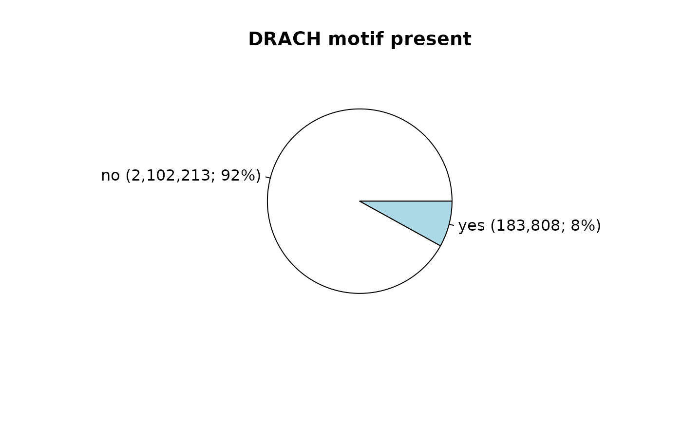

Use saveRDS(data_matrix, file = "data_matrix.rds") to store the current state. Use data_matrix <- readRDS("data_matrix.rds") to restore previous state.

Use NMF on Nanopore data

The learning part can be omitted. Use data(m6a_nmf_results) from Piechotta et al. (2021) and and continue to Visualize NMF.

Continue reading Overlap with miCLIP data, to understand how object m6a_nmf_results can be created.

Overlap with miCLIP data

Next, we use existing miCLIP data to train the model.

The data can be investigated with: data(m6a_miclip). It consists of 3 experiments:

Körtel et al. (2021),
Koh, Goh, and Goh (2019), and
Boulias et al. (2019) .

The column “experiments” indicates the source of a site.

Plot venn diagram of shared CLIP sites:

miclip_plt <- m6a_miclip %>%
  mutate(site = as.character(.)) %>%
  as.data.frame() %>%
  tidyr::separate_rows(experiments) %>%
  with(tapply(site, experiments, list)) %>%
  venn.diagram(
    filename = NULL,
    lwd = 1,
    cex = 0.5,
    fontfamily = "sans",
    cat.cex = 0.9,
    cat.default.pos = "outer",
    cat.fontfamily = "sans",
  )
grid.newpage()
grid.draw(miclip_plt)

We add miCLIP information to data_matrix:

data(m6a_miclip)

# Add region around site to miCLIP data
m6a_miclip_region <- extend(m6a_miclip, left = 2, right = 2)
m6a_miclip_region$experiments <- m6a_miclip$experiments

miclip_covered <- subsetByOverlaps(
  m6a_miclip_region,
  GRanges(rownames(data_matrix)),
  type = "equal"
)
data_matrix$experiments <- "-"
data_matrix[as.character(miclip_covered), "experiments"] <- miclip_covered$experiments

table(data_matrix$experiments)
#> 
#>                   -             Boulias     Boulias,Koertel Boulias,Koertel,Koh 
#>             2255751                8490                4966                2916 
#>         Boulias,Koh             Koertel         Koertel,Koh                 Koh 
#>                 850                7831                2249                2968

Next, we create the data matrix (corresponds to $X$ in $N \approx W H$) of sites that are contained in all three data sets: Boulias, Koertel, and Koh. It will be used to learn the modification patterns:

# retain sites that overlap with 3 miCLIP experiments

keep <- data_matrix$experiments == "Boulias,Koertel,Koh"
train_matrix <- data_matrix[keep, ]

table(train_matrix$DRACH)
#> 
#>  yes 
#> 2916

Compute factorizaion rank(s)

An important parameter in NMF is the factorization rank $r$ that defines the number of features to approximate $X$ - a similar parameter such as the number of clusters in the k-means algorithm. We will compute multiple factorizations with different values for $r$ and use surrogate measures to find an appropriate value.

Make sure that the data/train matrix ($X$) contains only numeric values before you start the factorization of $X$ to $W H$. The functions that does the calculations in JACUSA2helper is nmf_learn(x, mods), where x is the data/train matrix and mods is a GRanges object of known modifications.

Internally, JACUSA2helper uses the NMF package. Check NMF vignette for details on parameters. The default parameters in JACUSA2helper are set to nmf_args = list(rank = 2:10, nrun = 10, seed = 123456, .opt = "vp4"). For example argument .opt=pv3 instructs to use 3 cores - adjust the number according to your machine.

When using the default parameters, factorizations for rank $r \in {2, ..., 10}$ will be computed:

nmf_results <- learn_nmf(
  train_matrix %>% select(-c(motif, DRACH, experiments))
)
#> Compute NMF rank= 2  ... + measures ... OK
#> Compute NMF rank= 3  ... + measures ... OK
#> Compute NMF rank= 4  ... + measures ... OK
#> Compute NMF rank= 5  ... + measures ... OK
#> Compute NMF rank= 6  ... + measures ... OK
#> Compute NMF rank= 7  ... + measures ... OK
#> Compute NMF rank= 8  ... + measures ... OK
#> Compute NMF rank= 9  ... + measures ... OK
#> Compute NMF rank= 10  ... + measures ... OK
#> 
Runs: |                                                        
Runs: |                                                  |   0%
Runs: |                                                        
Runs: |==================================================| 100%
#> System time:
#>    user  system elapsed 
#>  27.862   3.942  22.604

The result nmf_results is a list that consists of the following data:

estim_r: Factorizations for x nmf_matrix; Factorization of x with r that maximizes estim_r$measures$silhouette.consensus and estim_r$measures$cophenetic chosen_rank; Optimal rank chosen_pattern; The pattern that has the highest score

In the next steps, we will evaluate the learned model by comparing it against a null model.

Visualize estimation of the ranks

We permutate the initial data and learn a randomized model:

nmf_random <- learn_nmf(
  train_matrix %>% 
    select(-c(motif, DRACH, experiments)) %>%
    randomize()
)
#> Compute NMF rank= 2  ... + measures ... OK
#> Compute NMF rank= 3  ... + measures ... OK
#> Compute NMF rank= 4  ... + measures ... OK
#> Compute NMF rank= 5  ... + measures ... OK
#> Compute NMF rank= 6  ... + measures ... OK
#> Compute NMF rank= 7  ... + measures ... OK
#> Compute NMF rank= 8  ... + measures ... OK
#> Compute NMF rank= 9  ... + measures ... OK
#> Compute NMF rank= 10  ... + measures ... OK
#> 
Runs: |                                                        
Runs: |                                                  |   0%
Runs: |                                                        
Runs: |==================================================| 100%
#> System time:
#>    user  system elapsed 
#>  25.921   4.013  20.669

In the following, we will compare the results for different factorizations on the original and randomized data:

# compare factorization on original and randomized data
plot(nmf_results$estim_r, nmf_random$estim_r)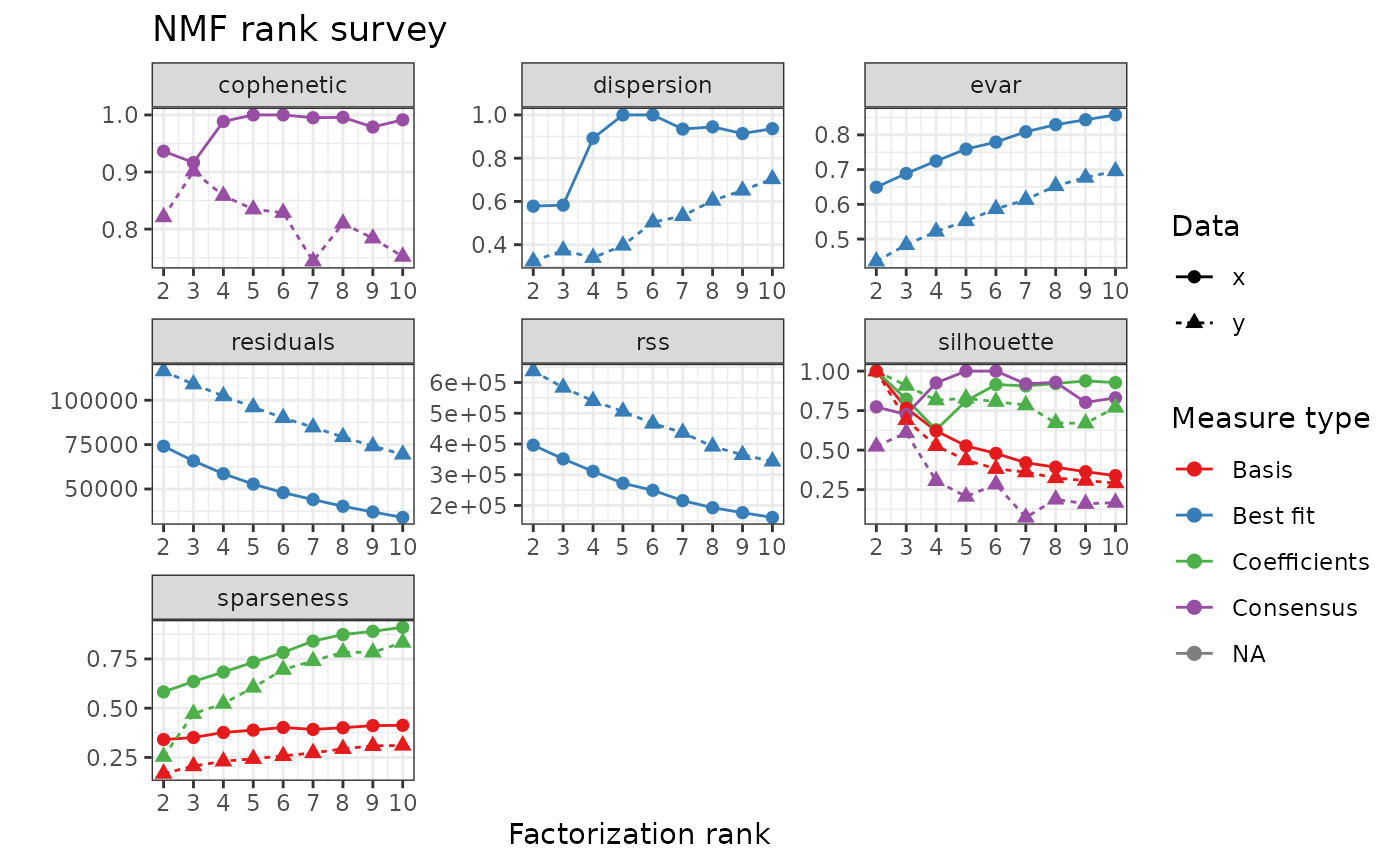

The optimal value of $r$ is the minimum rank for which rank Silhouette and Cophenetic is maximized.

Visualize NMF

Basis components

Plot properties of $W$.

basismap(nmf_results$nmf_matrix)

Mixture components

Plot properties of $H$.

coefmap(nmf_results$nmf_matrix)

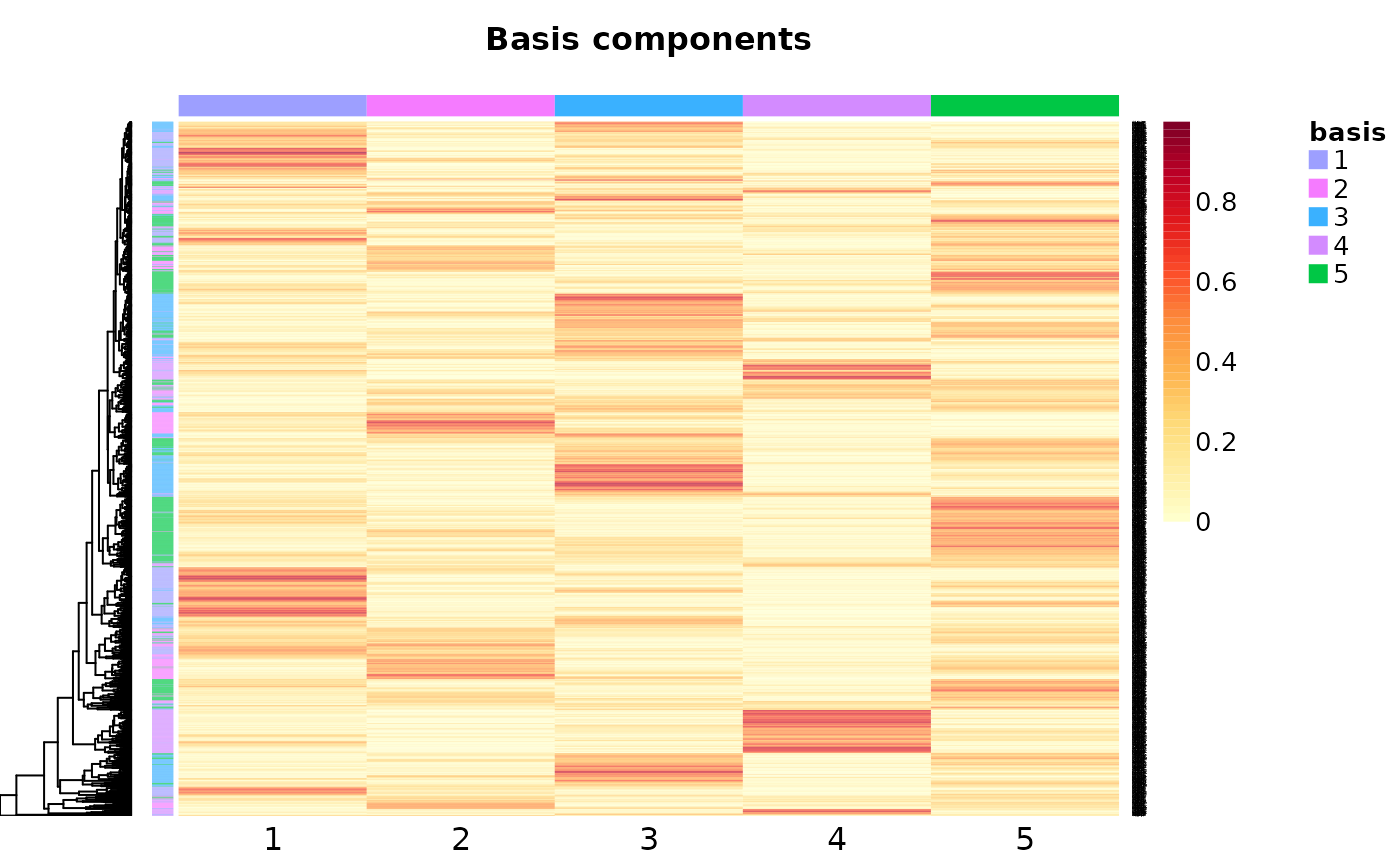
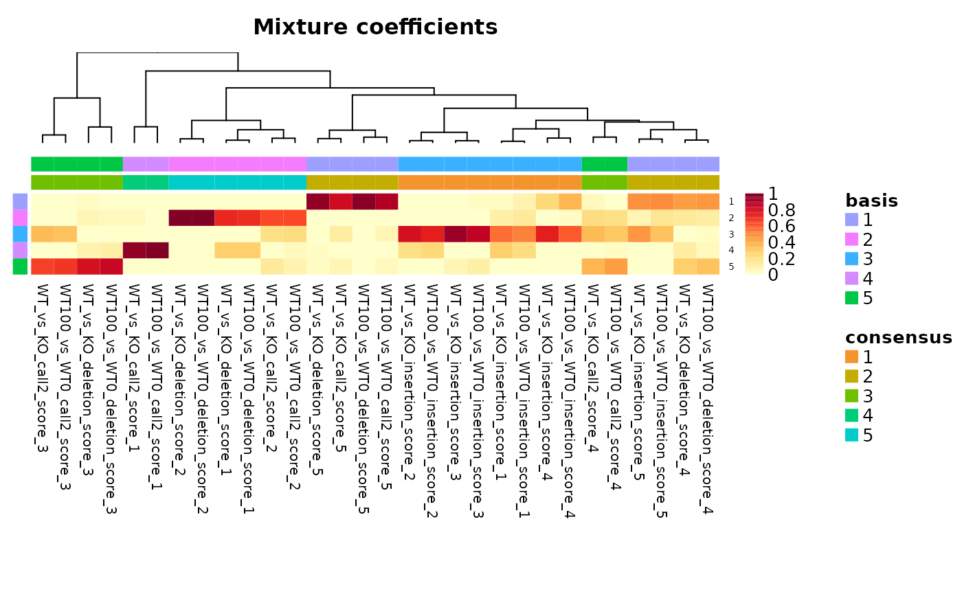
Visualize patterns

w <- basis(nmf_results$nmf_matrix)
# Table of number of best hits for each pattern"
pattern_instances <- apply(w, 1, function(x) {
    which(x == max(x))
  }
)
pattern_instance_tbl <- table(pattern_instances)

barplot(
  height = pattern_instance_tbl,
  names = 1:ncol(w),
  main = "NMF Patterns Scoring", 
  xlab = "Patterns", 
  ylab = "Membership Score (basis matrix)",
  ylim = range(pretty(c(0, pattern_instance_tbl)))
)

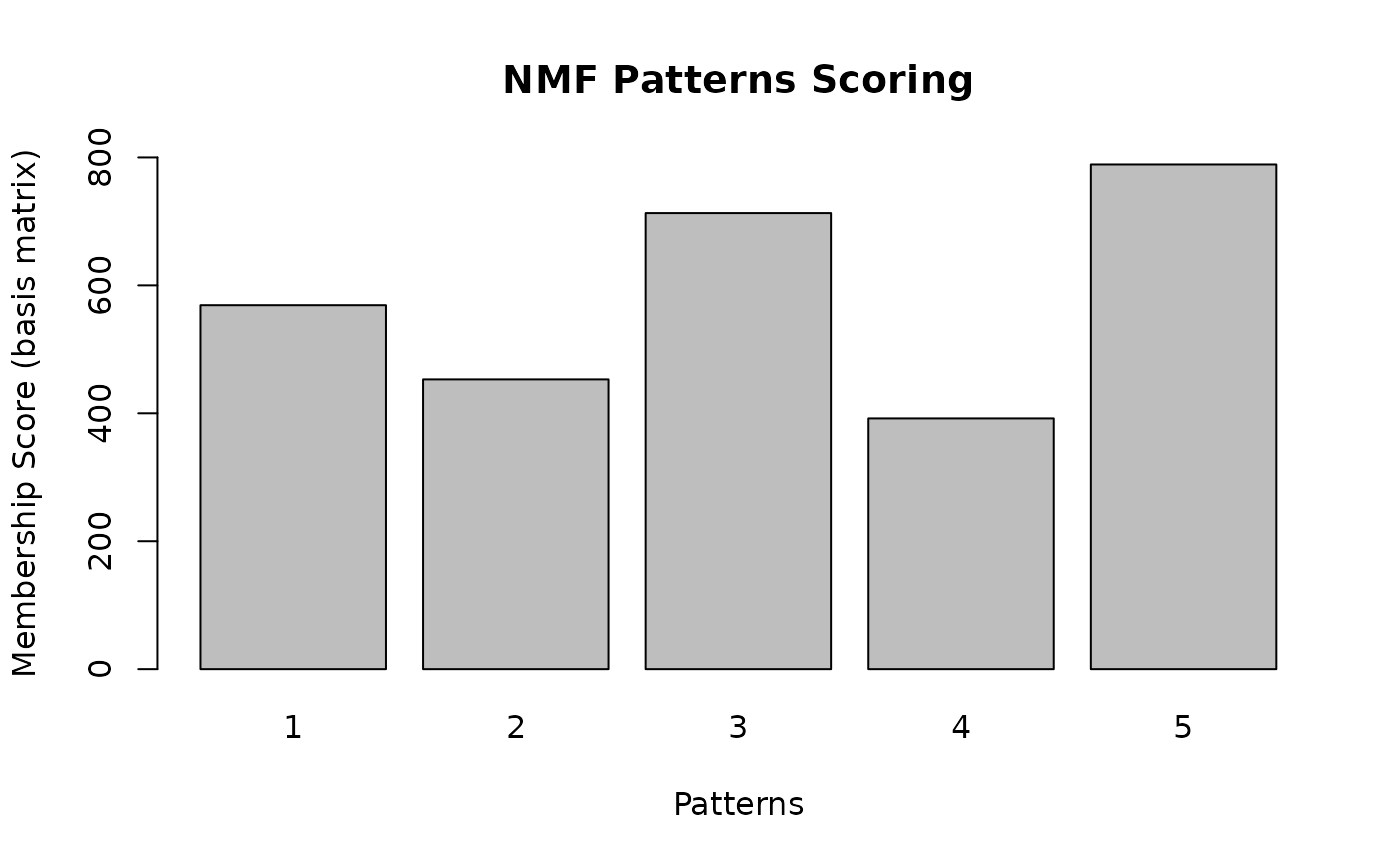
From this plot, we see that the highest score can observed for pattern:

nmf_results$chosen_pattern
#> [1] 5

Next, we visualize the sequence logos that correspond to calculated patterns in NMF.

h <- coef(nmf_results$nmf_matrix)

sequences <- lapply(1:nrow(h), function(k) {
  region_index <- rownames(train_matrix) %in% names(which(pattern_instances == k))
  return(train_matrix[region_index, "motif"])
})
names(sequences) <- paste0("Pattern ", 1:nrow(h))
ggseqlogo::ggseqlogo(sequences)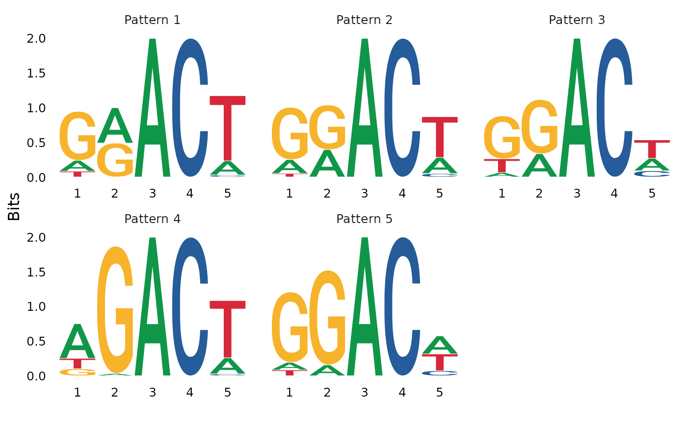

Finally, we plot profiles for each pattern and experiment (meta condition):

as.data.frame(h) %>% 
  mutate(pattern = 1:nrow(.)) %>% 
  tidyr::pivot_longer(
    -pattern, 
    names_to = c("Exp", "Score", "Pos"), 
    names_pattern = "(WT_vs_KO|WT100_vs_WT0)_(call2_score|deletion_score|insertion_score)_([1-5]+)"
  ) %>% 
  mutate(score = gsub("_score$", "", Score)) %>% 
  ggplot(aes(x = Pos, y = value, fill = Score)) + 
    geom_bar(stat = "identity") + 
    xlab("Position in motif\n-NN A NN-") +
    ylab("") +
    facet_grid(Exp ~ pattern, labeller = label_both)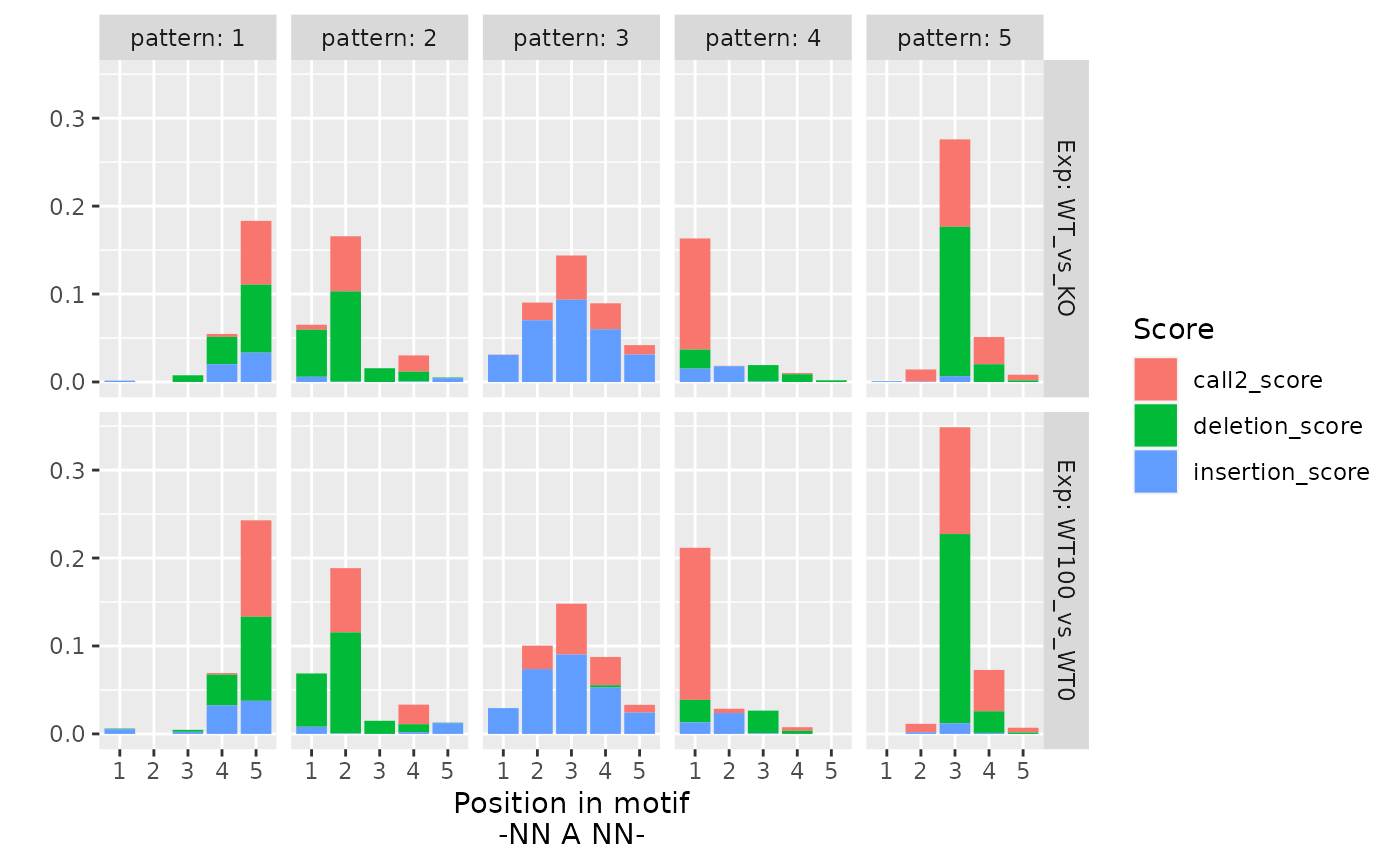

Prediction

We evaluate the factorization on the previously introduced miCLIP data. We use all sites. WARNING! Make sure that the order of columns is correct - use create_data().

score_matrix <- predict_mods(
  data_matrix %>% select(-c(motif, DRACH, experiments)), 
  nmf_results
)

score_matrix consists of columns scores for each pattern and the score for the chosen pattern (in this case: NMF5 = score). We add meta information from data_matrix to score_matrix.

score_matrix <- cbind(score_matrix, data_matrix[, c("motif", "DRACH", "experiments")])

colnames(score_matrix)
#> [1] "NMF1"        "NMF2"        "NMF3"        "NMF4"        "NMF5"       
#> [6] "score"       "motif"       "DRACH"       "experiments"

Sort score_matrix by column score - the best predictions will appear in the upper part of matrix.

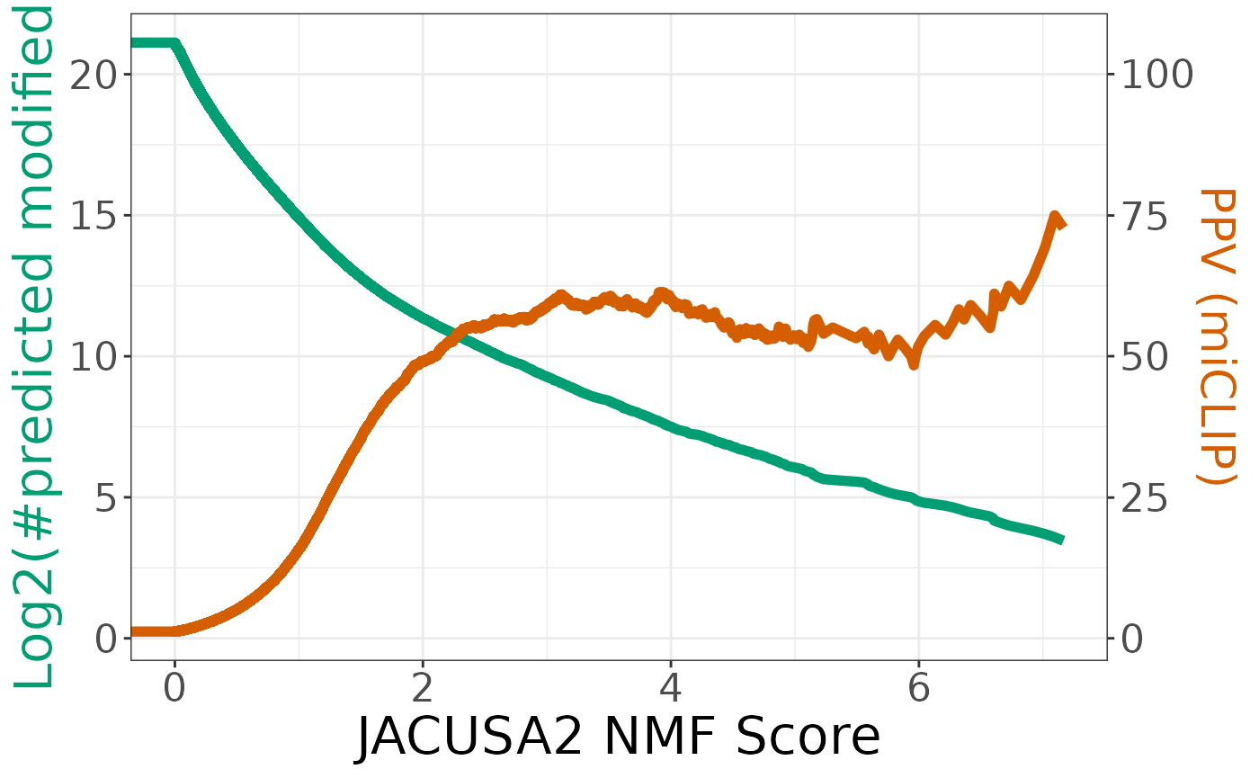
Evaluation

score_matrix$clip <- if_else(score_matrix$experiments != "-", "CLIP", "No Clip")
score_matrix$type <- "-"

train <- score_matrix$experiments == "Boulias,Koertel,Koh"
score_matrix$type[train] <- "train"
score_matrix$type[!train] <- "evaluate"

table(score_matrix$clip, score_matrix$type)
#>          
#>           evaluate   train
#>   CLIP       27354    2916
#>   No Clip  2255751       0

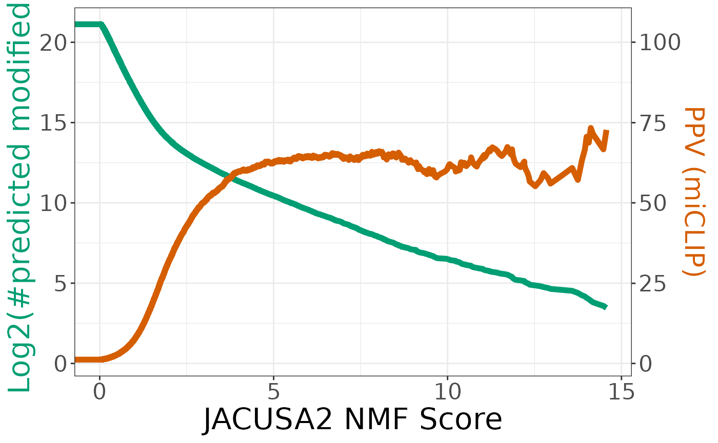
test_matrix <- score_matrix[score_matrix$type == "evaluate", ]
r <- roc(
  ifelse(test_matrix[, "clip"] == "CLIP", 1, 0), 
  test_matrix[, "score"]
)
#> Setting levels: control = 0, case = 1
#> Setting direction: controls < cases

coordinates <- coords(r, x = "all", input = "threshold", ret = c("threshold","ppv","tpr","tp", "tn","fp","fn"))
coordinates$sum <- log2(coordinates$tp + coordinates$fp)
coordinates$ppv <- coordinates$ppv * 20
coordinates <- coordinates[which(coordinates$sum > log2(10)),]

ggplot(coordinates, aes(x = threshold)) +  
  geom_line(aes(y = sum), size = 2, color = "#009E73") + 
  geom_line(aes(y = ppv), size = 2, color = "#D55E00") +
  scale_y_continuous(
    # Features of the first axis
    name = "Log2(#predicted modified)",
    # Add a second axis and specify its features
    sec.axis = sec_axis(~.*5, name = "PPV (miCLIP)")
  ) +  
  scale_x_continuous(name = "JACUSA2 NMF Score") + 
  theme_bw() +
  theme(
    axis.title.x = element_text(size = rel(2)),      
    axis.title.y = element_text(color = "#009E73", size = rel(2)),
    axis.title.y.right = element_text(color = "#D55E00", size = rel(0.9)), 
    axis.text = element_text(size = rel(1.5))
  )

Prediction on 1 experiment

In the following we will show how to predict modification sites on only one experiment.

Prepare data

We will predict modification sites only on WT vs KO from the previous example. If you have your own data, follow the steps above until create_data(). Here, we will modify the existing data_matrix:

WT_vs_KO_data <- cbind(
  data_matrix[, grep("^WT_vs_KO", colnames(data_matrix))],
  data_matrix[, c("motif", "DRACH", "experiments")]
)
WT_vs_KO_data$clip <- if_else(WT_vs_KO_data$experiments != "-", "CLIP", "No Clip")
WT_vs_KO_data$type <- "-"

train <- WT_vs_KO_data$experiments == "Boulias,Koertel,Koh"
WT_vs_KO_data$type[train] <- "train"
WT_vs_KO_data$type[!train] <- "evaluate"

Reduce coef

We need to adjust the coefficient matrix and combine the coefficients from WT vs KO and WT100 vs WT0.

nmf_reduced <- reduce_coef(nmf_results, meta_conds)
names(nmf_reduced)
#> [1] "estim_r"        "chosen_rank"    "chosen_pattern" "nmf_matrix"    
#> [5] "reduced_coef"

This will calculate the mean of the coefficients and add the result as reduced_coef to nmf_results.

Prediction

WT_vs_KO_pred <- predict_mods(
  select(WT_vs_KO_data, -c(motif, DRACH, experiments, clip, type)),
  nmf_reduced
)
WT_vs_KO_pred <- cbind(WT_vs_KO_pred, WT_vs_KO_data[, c("clip", "type")])

Column score, can be used to sort the prediction.

Evaluate

We repeat the evaluation now on WT vs KO and the reduced coefficient matrix on.

WT_vs_KO_test <- WT_vs_KO_pred[WT_vs_KO_pred$type == "evaluate", ]
WT_vs_KO_roc <- roc(
  ifelse(WT_vs_KO_test[, "clip"] == "CLIP", 1, 0), 
  WT_vs_KO_test[, "score"]
)
#> Setting levels: control = 0, case = 1
#> Setting direction: controls < cases

WT_vs_KO_coords <- coords(WT_vs_KO_roc, x = "all", input = "threshold", ret = c("threshold","ppv","tpr","tp", "tn","fp","fn"))
WT_vs_KO_coords$sum <- log2(WT_vs_KO_coords$tp + WT_vs_KO_coords$fp)
WT_vs_KO_coords$ppv <- WT_vs_KO_coords$ppv * 20
WT_vs_KO_coords <- WT_vs_KO_coords[which(WT_vs_KO_coords$sum > log2(10)),]

ggplot(WT_vs_KO_coords, aes(x = threshold)) +  
  geom_line(aes(y = sum), size = 2, color = "#009E73") + 
  geom_line(aes(y = ppv), size = 2, color = "#D55E00") +
  scale_y_continuous(
    # Features of the first axis
    name = "Log2(#predicted modified)",
    # Add a second axis and specify its features
    sec.axis = sec_axis(~.*5, name = "PPV (miCLIP)")
  ) +  
  scale_x_continuous(name = "JACUSA2 NMF Score") + 
  theme_bw() +
  theme(
    axis.title.x = element_text(size = rel(2)),      
    axis.title.y = element_text(color = "#009E73", size = rel(2)),
    axis.title.y.right = element_text(color = "#D55E00", size = rel(0.9)), 
    axis.text = element_text(size = rel(1.5))
  )

References

Boulias, Konstantinos, Diana Toczydłowska-Socha, Ben R. Hawley, Noa Liberman, Ken Takashima, Sara Zaccara, Théo Guez, et al. 2019. “Identification of the m6Am Methyltransferase PCIF1 Reveals the Location and Functions of m6Am in the Transcriptome.” Molecular Cell 75 (3): 631–643.e8. https://doi.org/10.1016/j.molcel.2019.06.006.

Koh, Casslynn W. Q., Yeek Teck Goh, and W. S. Sho Goh. 2019. “Atlas of Quantitative Single-Base-Resolution N6-Methyl-Adenine Methylomes.” Nature Communications 10 (1): 5636. https://doi.org/10.1038/s41467-019-13561-z.

Körtel, Nadine, Cornelia Rücklé, You Zhou, Anke Busch, Peter Hoch-Kraft, F X Reymond Sutandy, Jacob Haase, et al. 2021. “Deep and Accurate Detection of m6A RNA Modifications Using miCLIP2 and m6Aboost Machine Learning.” Nucleic Acids Research 49 (16): e92–92. https://doi.org/10.1093/nar/gkab485.

Piechotta, Michael, Qi Wang, Janine Altmüller, and Christoph Dieterich. 2021. “RNA Modification Mapping with JACUSA2,” July. https://doi.org/10.1101/2021.07.02.450888.

Christoph Dieterich, Michael Piechotta

2023-01-18

Non-negative Matrix Factorization

General workflow

Pre-processing

Read

Filter

Add meta condition

Add reference sequence information

Create matrix \(X\)

Generalize

Create data matrix

Add sequence

Use NMF on Nanopore data

Overlap with miCLIP data

Compute factorizaion rank(s)

Visualize estimation of the ranks

Visualize NMF

Basis components

Mixture components

Visualize patterns

Prediction

Evaluation

Prediction on 1 experiment

Prepare data

Reduce coef

Prediction

Evaluate

References