Application to epitranscriptomics

Introduction

The pulseR package may be adapted for analysis of experimental approaches, which are similar to the metabolic labelling in having several related fractions. For example, RNA modification level can be measured on the basis of immunoprecipitation (IP) using antibodies against of modified nucleotisides, e.g. anti-m\(^6\)A or anti-m\(^5\)C IgG.

Here we consider an example of the LAIC-seq approach, published here

Molinie, Benoit, et al. “m(6)A-LAIC-seq reveals the census and complexity of the m(6)A epitranscriptome.” Nature methods 13.8 (2016): 692.

The data consists of three fractions:

total (“input”) \(\leftarrow\) the original pool
pull-down (“elution”) \(\leftarrow\) m\(^6\)A modified RNA
flow-through (“supernatant”) \(\leftarrow\) m\(^6\)A nonmodified RNA.

Since during library preparation, usually the probes are normalised to the same amount (e.g. 100ng), it is important to recover the original relation between the pull-down, flow-through and the total fractions. One may whether

use external molecules for normalisation (e.g. ERCC spike-ins or RNA from another species). The approaches are
1. external spike-in molecules are added in known (e.g. equal) proportion right after the purification (\(\leftarrow\) approach in the original paper). One must prove experimentally, that efficiency of separation is high (negligible cross-contamination)
2. nonmodified and modified (e.g. m\(^6\)A\(^+\) RNA) spike-ins are before the purification
estimate relations between fractions during model fitting ( \(\leftarrow\) this example)

The task of normalisation and the model fitting can be illustrated with the following figure:

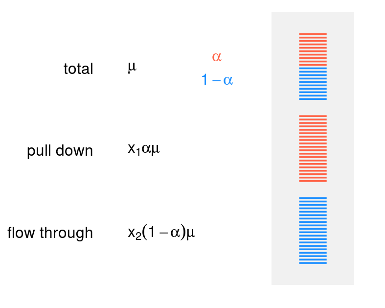
Considering the total sample as a reference, with denote the expression level of a given gene as \(\mu\). Then if \(\alpha\) is proportion of modified molecules (a value between 0 and 1), the amount of the modified molecules in the total sample is \(\alpha\mu\) and amount of the nonmodified molecules is \((1 - \alpha)\mu\).

However, normalisation of material for library preparation affects the expected read counts in both fractions, and the task is to recover additional normalisation factors \(x_1\) and \(x_2\) (see figure), in such a way, that the read counts can be explained by the model. The coefficients \(x_1\) and \(x_2\) are shared between all the genes, and the expression level and modification level are gene-specific.

Analysis

Get and prepare the data

Thanks to the authors, the paper is accompanied by the supplementary count table, which makes reproducibility much easier. In this subsection, preliminary steps for data preparation are discussed. Download the table with read counts and results from the publisher’s site:

library(openxlsx)
dataURL <- "https://media.nature.com/original/nature-assets/nmeth/journal/v13/n8/extref/nmeth.3898-S2.xlsx"
laicSeqData <- read.xlsx(dataURL)

Prepare the condition table and the count table:

counts <- laicSeqData[, -(1:10)]
rownames(counts) <- laicSeqData$Gene_ID

conditions <- do.call(rbind, strsplit(names(counts), "_"))
conditions <- data.frame(conditions[,3:1], stringsAsFactors = FALSE)
names(conditions) <- c("fraction", "run", "cells")
conditions$sample <- names(counts)

conditions$fraction <- c(
 "input" = "total",
 "elu"   = "pull-down",
 "sup"   = "flow-through")[conditions$fraction]

## In this example we use only the "GM" cells data set
cellTypeIndex <- conditions$cells == "GM"
byFraction <- order(conditions$fraction[cellTypeIndex], decreasing = TRUE)

counts     <- counts[, cellTypeIndex][,byFraction]
conditions <- conditions[cellTypeIndex,][byFraction,]

knitr::kable(conditions, row.names = FALSE)

fraction	run	cells	sample
total	sp1	GM	GM_sp1_input_pairs
total	sp2	GM	GM_sp2_input_pairs
pull-down	sp1	GM	GM_sp1_elu_pairs
pull-down	sp2	GM	GM_sp2_elu_pairs
flow-through	sp1	GM	GM_sp1_sup_pairs
flow-through	sp2	GM	GM_sp2_sup_pairs

The count table looks like

	GM_sp1_input_pairs	GM_sp2_input_pairs	GM_sp1_elu_pairs	GM_sp2_elu_pairs	GM_sp1_sup_pairs	GM_sp2_sup_pairs
ENSG00000167634	103	140	43	42	143	201
ENSG00000104951	2951	3823	5929	5244	2521	4282
ENSG00000116096	112	130	153	172	87	150
ENSG00000137496	741	787	1350	1145	476	578
ENSG00000123933	398	536	281	263	456	681
ENSG00000266728	747	810	738	597	756	724

Which parametrisation to use?

There are several ways to report the methylation level:

as a proportion \(\alpha\) of the molecules, which are trapped by the antibodies.
In this case, \(\alpha\) is in [0,1] interval.
as a ratio of modified / nonmodified molecules.
It is equal to \(\alpha/(1 - \alpha)\) and is in \([0,\infty)\) interval
as the logarithm of odds, \(\gamma = \log\left(\dfrac{\alpha}{1 - \alpha}\right)\) \(\leftarrow\) we are here.
It can take all the values from \((-\infty, \infty)\).

Out of these three parameters, only the log(odds) is symmetrical in respect to the modified and unmodified molecules quantities. If, for example, the level of modification increases from 80% to 90%, it is only a mild change in the proportion (1.125-fold), but the amount of nonmodified molecules decreased from 20% to 10%, which is 2-fold decrease. Hence, the extent of the difference depends on the molecule type, we are considering.

In contrast, if we swap the labels of the molecules in the log(odds), it results only in change of the sign, but not the absolute value:

lor <- function(a) log(a/(1 - a))
lor(.9) - lor(.8) # change from 80% to 90%
#> [1] 0.8109302
lor(.1) - lor(.2) # change from 20% to 10%
#> [1] -0.8109302

It is always good to keep gene-specific parameters at the same scale, since currently the stopping criteria for fitting depends on the absolute changes in parameter values between iterations. That it is why, if the log(odds) is used, it is better to describe the expression level at the logarithmic scale, i.e. mean read count is \[\text{[total]} = e^{\mu}\] and the amount of modified molecules is \[\text{[modified]} = e^{\mu + \gamma} / (1 + e^{\gamma}).\]

Model definition

In this workflow, we use the parametrisation based on the log(odds). To have parameters of similar scale, the expression level is modelled at the logarithmic scale, i.e. mean read count in the total fraction is exp(mu).

To use the pulseR package, we need to define these formulas and describe, how the read counts in different conditions are related to the formulas:

library(pulseR)
formulas <- MeanFormulas(
  total       = exp(mu),
  modified    = exp(y + mu) / (1 + exp(y)),
  nonmodified = exp(mu) / (1 + exp(y))
)
formIndexes <- list(
  "total"        = "total",
  "pull-down"    = "modified",
  "flow-through" = "nonmodified"
)

It is important to note, that here we neglect cross-contamination, as in the paper it was experimentally shown, that the purification procedure is very efficient, which results in high quality separation.

Alternatively, one may use spike-ins for estimation of the cross-contamination levels and relation of fractions to each other.

To keep computations light, we use only highly expressed genes, using mean read count in the total fraction for filtering:

expressionRank <- rank(
  -rowMeans(counts[, conditions$fraction == "total"]))
highExp <- expressionRank < 501

Now we prepared everything for the PulseData object initialisation:

pd <- PulseData(counts = counts[highExp,],
                conditions = conditions[, 1,  drop = FALSE],
                formulas = formulas,
                formulaIndexes = formIndexes,
                groups = ~fraction)

Fitting options

The model is fitted using the optimisation routine “L-BFGS-B”, which requires boundaries for the parameters. In this case, there are following parameters to fit:

gene specific: logarithmic expression level \(\mu\) and the log(odds) \(\gamma\) for RNA modification
size parameter for the negative binomial distribution (shared between all the genes)
normalisation factors (shared between the samples from the same condition, i.e. a single factor for e.g. “pull-down” samples). Alternatively, every sample can be attributed with its own normalisation factor, if, for example, efficiency of purification is varies between repetitions (batches).


lbNormFactors <- list(
  "total"        = .1,
  "pull-down"    = .1,
  "flow-through" = .1
)
ubNormFactors <- list(
  "total"        = 2e1,
  "pull-down"    = 2e1,
  "flow-through" = 2e1
)

opts <- setBoundaries(list(
  mu = log(c(.1, 1e8)),
  y = c(-5,5),
  size = c(.1,1e6)),
  normFactors = list(lbNormFactors, ubNormFactors)
)
## Set stopping criteria for fitting:
## absolute difference between iterations must be not higher than 0.1 for
## the parameters (mu and y) and the normalisation factors
opts <- setTolerance(params = .1, 
                     options = opts,
                     normFactors = .1,
                     logLik = 1 # minimal absolute difference for the logLikelihood
)
opts$verbose <- "silent"
opts$resultRDS <- NULL # a path to save the result after every iteration
opts$cores <- 3

To start model fitting, it can be beneficial to initialise the parameters close to their expected values: for example, the parameter mu must be near the logarithm of the read counts in the total fractions.

The normalisation factors will be fitted as well, except for the very first item: it is the reference for all other samples and will be fixed to 1 identifiability.

# create a list of needed structure and then adjust the values
pars <- initParameters(list(), c("mu", "y"), pd, opts)
pars$mu <- log(pd$counts[, 1] + 1)
pars$y[] <- 0 # corresponds to 50% methylation
pars$size <- 1000
pars$normFactors[[2]] <- 2
pars$normFactors[[3]] <- 2

## look inside the initial guess
str(pars)
#> List of 4
#>  $ mu         : Named num [1:500] 8.57 9.39 8.66 8.63 9.14 ...
#>   ..- attr(*, "names")= chr [1:500] "ENSG00000171992" "ENSG00000245532" "ENSG00000258486" "ENSG00000175265" ...
#>  $ y          : num [1:500] 0 0 0 0 0 0 0 0 0 0 ...
#>  $ size       : num 1000
#>  $ normFactors:List of 3
#>   ..$ : num 5.91
#>   ..$ : num 2
#>   ..$ : num 2

Finally, run the fitting using the initial values, options and the data provided:

result <- fitModel(pd, pars, opts)

Results

We may compare how the model prediction and the raw counts relate to each other, using the predictExpression function:

pr <- predictExpression(result, pd)

plot(as.vector(pd$counts) + .5,
 as.vector(pr$predictions) + .5,
 log='xy',
 cex = .3,
 xlab = "experiment",
 ylab = "model")
abline(0,1,col = 2, lwd = 2)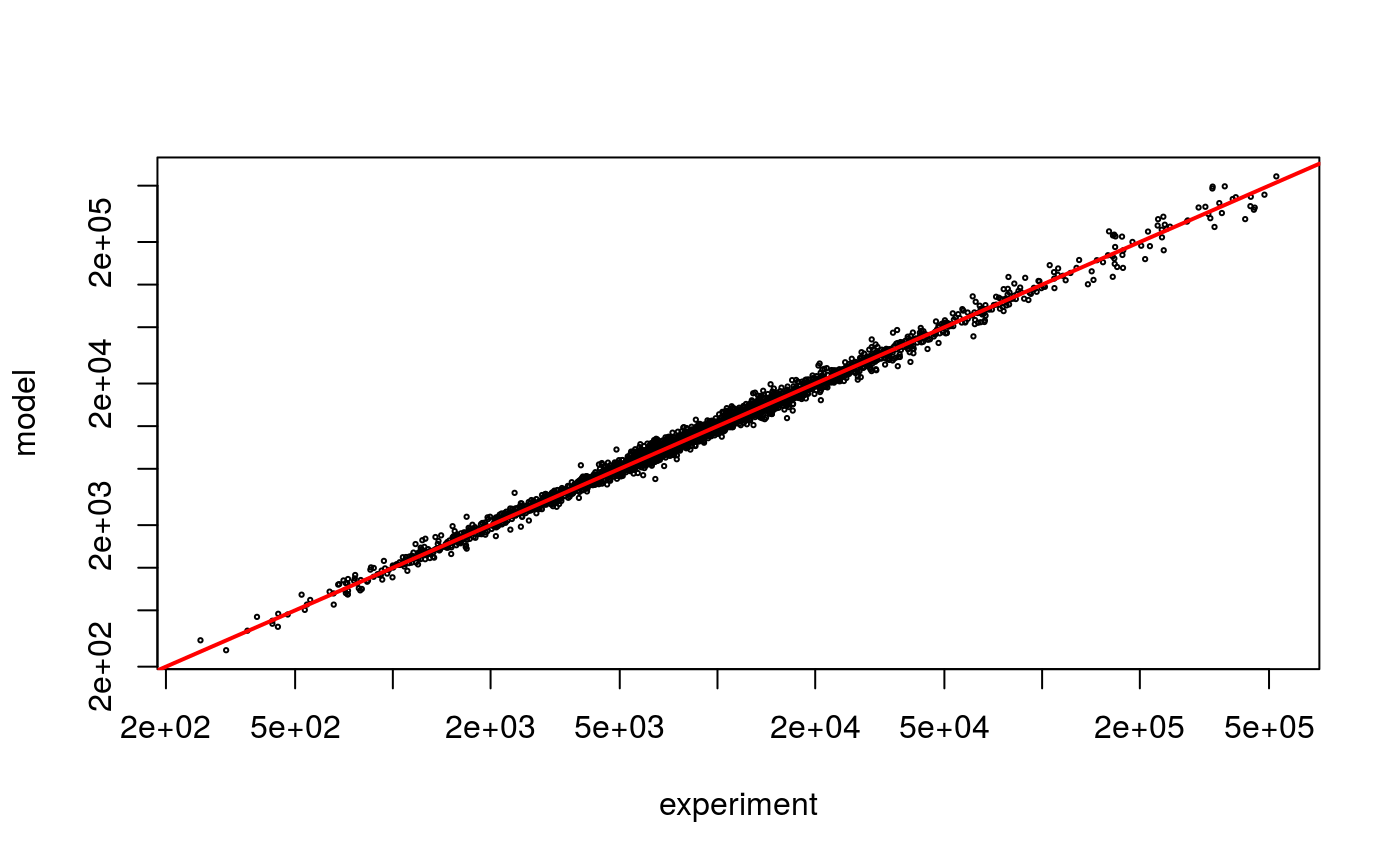

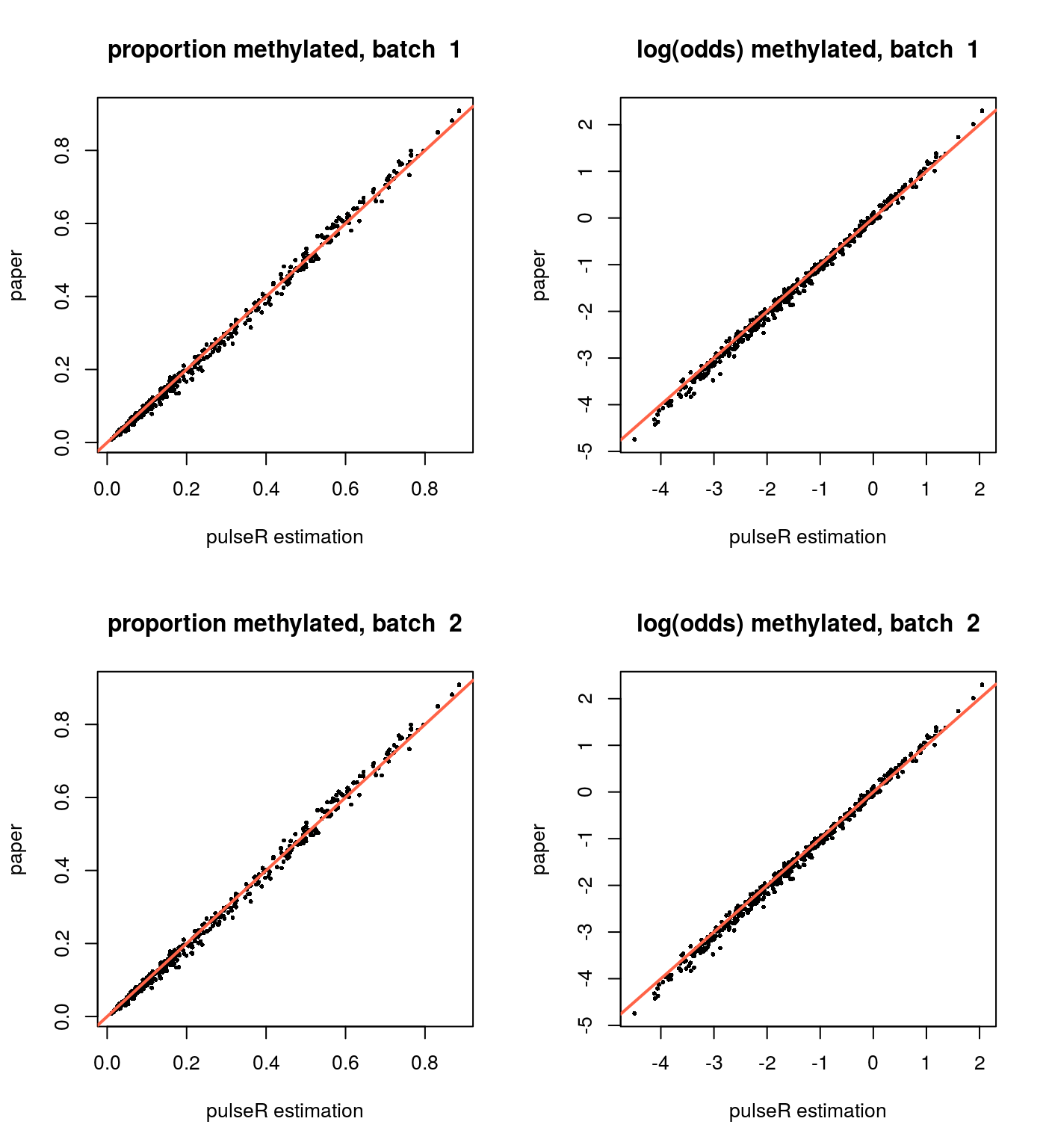
In addition, in the paper supplementary the estimations for the methylation levels are available for two experiment repetitions. It is interesting to compare the pulseR estimations based on the both repetitions and the estimations from the paper.

Since we use only a subset of the data and a different way to normalise the fractions, it affects the estimations of the methylation level, hence a global bias between these two results can be observed, i.e. estimations will be shifted to higher or lower values. It complicates comparison of the results from, for example, different studies, and further development is needed in order to tackle this problem.

paperResults <- laicSeqData[highExp,c(1,6,7)]
head(paperResults)
#>     Gene_symbol GM_sp1_m6A_level GM_sp2_m6A_level
#> 12        SYNPO        0.4965471        0.5406506
#> 56        NEAT1        0.7849989        0.7952290
#> 60       RN7SL1        0.3111133        0.3156488
#> 122     GOLGA8A        0.5621528        0.5491124
#> 204       MACF1        0.5904389        0.5557059
#> 218        MAP4        0.6212910        0.6074293

or2alpha <- function(or) exp(or) / (1 + exp(or))
par(mfrow = c(2,2))
plotCompare <- function(...) {
  plot(cex = .5, pch = 16, ...)
  abline(0, 1, col = "tomato", lwd = 2)
}
for(i in 1:2) {
  plotCompare(or2alpha(result$y), paperResults[,2],
    xlab = "pulseR estimation",
    ylab = "paper",
    main = paste("proportion methylated, batch ", i))
  plotCompare(result$y, lor(paperResults[,2]),
    xlab = "pulseR estimation",
    ylab = "paper",
    main = paste("log(odds) methylated, batch ", i))
}

Confidence intervals

In addition to the estimations, one usually is interested to have confidence intervals for making inference about the parameter values, for example, to compare between different conditions.

The function ciGene allows to estimate CI for the gene specific parameters. In this case, uncertainty from the normalisation factors is neglected and the profile of the likelihood is computed assuming the normalisation factors and the size parameter to be fixed.

opts$replicates <- 3
cis <- ciGene(parName = "y",
              geneIndexes = seq_along(result$y),
              par = result,
              pd = pd,
              options = opts,
              interval = c(-5, 5),
              confidence = .95
)

Here we gather the results into a data.frame and plot the confidence intervals and the estimated values. The genes are sorted by their m6A level:


dat <- data.frame(
  y = result$y,
  mu = result$mu,
  y.min = cis[,1],
  y.max = cis[,2]
)

dat$paperAvg <- rowMeans(paperResults[,2:3])
dat$lor.paperAvg <- lor(dat$paperAvg)

par(mfrow = c(2,1), mar = c(5,5,4,2))
o <- order(dat$y)
i <- seq_along(dat$y)
plot(x = i, y = dat$y[o], type = "n",
  xlab = expression(paste(m^6, A, "  rank")),
  ylab = expression(paste(m^6, A, " log(odds)")),
  cex.lab = 1.2
)
lines(x = i, y = dat$y.max[o], col = "dodgerblue")
lines(x = i, y = dat$y.min[o], col = "dodgerblue")
points(x = i, y = dat$y[o], cex = .3)

plot(x = i, y = or2alpha(dat$y[o]), type = "n",
  xlab = expression(paste(m^6, A, "  rank")),
  ylab = expression(paste(m^6, A, "  proportion")),
  cex.lab = 1.2
)
lines(x = i, y = or2alpha(dat$y.max[o]), col = "dodgerblue")
lines(x = i, y = or2alpha(dat$y.min[o]), col = "dodgerblue")
points(x = i, y = or2alpha(dat$y[o]), cex = .3)

On bias in estimations

As it was mentioned before, the normalisation may have high influence on the estimated values, which can shift the absolute values to higher or lower values, although the ranking is much less affected. To illustrate how estimations compare to each other, I add to the previous plot the average of the two estimations from the paper (red dots):

par(mar = c(5,5,4,2))
plot(x = i, y = dat$y[o], type = "n",
  xlab = expression(paste(m^6, A, "  rank")),
  ylab = expression(paste(m^6, A, " log(odds)")),
  cex.lab = 1.2
)
lines(x = i, y = dat$y.max[o], col = "dodgerblue")
lines(x = i, y = dat$y.min[o], col = "dodgerblue")
points(x = i, y = dat$y[o], cex = .3)
points(x = i, y = dat$lor.paperAvg[o], cex = .3, col = "tomato")
legend("topright", legend = c("pulseR", "paper"), col = c("black", "tomato"),
  lty = 1)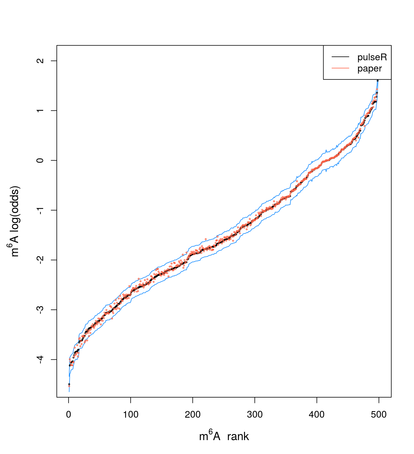

sessionInfo()
#> R version 3.4.0 (2017-04-21)
#> Platform: x86_64-pc-linux-gnu (64-bit)
#> Running under: Ubuntu 16.04.5 LTS
#> 
#> Matrix products: default
#> BLAS: /usr/lib/openblas-base/libblas.so.3
#> LAPACK: /usr/lib/libopenblasp-r0.2.18.so
#> 
#> locale:
#>  [1] LC_CTYPE=en_US.UTF-8       LC_NUMERIC=C              
#>  [3] LC_TIME=de_DE.UTF-8        LC_COLLATE=en_US.UTF-8    
#>  [5] LC_MONETARY=de_DE.UTF-8    LC_MESSAGES=en_US.UTF-8   
#>  [7] LC_PAPER=de_DE.UTF-8       LC_NAME=C                 
#>  [9] LC_ADDRESS=C               LC_TELEPHONE=C            
#> [11] LC_MEASUREMENT=de_DE.UTF-8 LC_IDENTIFICATION=C       
#> 
#> attached base packages:
#> [1] stats     graphics  grDevices utils     datasets  methods   base     
#> 
#> other attached packages:
#> [1] pulseR_1.0.3
#> 
#> loaded via a namespace (and not attached):
#>  [1] Rcpp_0.12.19       knitr_1.20         xml2_1.2.0        
#>  [4] magrittr_1.5       roxygen2_6.1.0     MASS_7.3-50       
#>  [7] R6_2.3.0           rlang_0.2.2        stringr_1.3.1     
#> [10] highr_0.7          tools_3.4.0        htmltools_0.3.6   
#> [13] commonmark_1.6     yaml_2.2.0         rprojroot_1.3-2   
#> [16] digest_0.6.18      assertthat_0.2.0   pkgdown_1.1.0.9000
#> [19] crayon_1.3.4       fs_1.2.6           memoise_1.1.0     
#> [22] evaluate_0.12      rmarkdown_1.10     stringi_1.2.4     
#> [25] compiler_3.4.0     desc_1.2.0         backports_1.1.2

Uvarovskii Alexey

17-10-2018