Overview
The workflow consists of defining the data object, setting fitting options and fitting itself:
library(pulseR)
...
# define the data
pd <- PulseData(...)
# set options
opts <- setTolerance(...)
opts <- setBoundaries(..., opts)
# define first parameter guess
initPars <- initParameters(...)
# fit the model
fit <- fitModel(pd, initPars, opts)
PulseData object
In the pulseR package, we keep all inial data in the PulseData structure (S3 class). When the information about read counts, conditions and the model is defined, one can create the object with a line as
library(pulseR)
attach(pulseRSpikeinsData)
pd <- PulseData(counts, conditions, formulas, formulaIndexes, spikeins)
Counts
The read counts must be delivered as an integer matrix. The rownames may describe the gene names and the column order corresponds to the sample order in the condition matrix (see below)
counts[c(1:5, 50:55), 1:4]
##         total_fraction total_fraction total_fraction pull_down
## gene_1            1006            983           1005      1859
## gene_2            1984           1975           1992      3214
## gene_3            2914           2971           3049      4930
## gene_4            4106           4012           3839      7377
## gene_5            5083           5240           4915      8455
## gene_50          49745          50289          50003     80099
## gene_51          50713          52207          50233     94670
## gene_52          51829          51490          51292     87236
## gene_53          53077          52261          54400     96165
## gene_54          52626          52373          53856    102734
## gene_55          55412          55741          55124     89592
Condition matrix
The information about samples must be described in the condition matrix. It is obligatory that the row order corresponds to the column order in the count matrix. Time or other sample-specific variable are defined here.
conditions
##                 fraction time
## sample_1  total_fraction    1
## sample_2  total_fraction    2
## sample_3  total_fraction    3
## sample_4       pull_down    1
## sample_5       pull_down    2
## sample_6       pull_down    3
## sample_7  total_fraction    1
## sample_8  total_fraction    2
## sample_9  total_fraction    3
## sample_10      pull_down    1
## sample_11      pull_down    2
## sample_12      pull_down    3
Formulas
The design of the experiment defines how different fractions evolve with the time. Let us consider the chase experiment, when the labelled molecules are being only degraded and the unlabelled molecules are synthesised and degraded:
formulas <- MeanFormulas(
  total      =  mu,
  labelled   =  mu * exp(-d * time),
  unlabelled =  mu * (1 - exp(-d * time))
)
Although the expression level in the form of mean read count is easier for perception, it can be better to model it at the logarithmic scale. In this case, the mean read counts is exp(mu), and the degradation rate d and logarithm of mean read count mu have values of the same scale, i.e. unit changes in d * time or mu result in similar changes in the expected read number:
formulas <- MeanFormulas(
  total      =  exp(mu),
  labelled   =  exp(mu - d * time),
  unlabelled =  exp(mu) * (1 - exp(-d * time))
)
In the mathematical form, it looks like \[ \begin{align} \text{[total]} &= e^\mu\\ \text{[labelled]} &= e^{\mu - d\cdot t}\\ \text{[unlabelled]} &= e^{\mu}\left(1 - e^{-d\cdot t}\right) \end{align} \]
In this vignette we use the logarithm of the mean read expression!
It is important to note, that one should not forget to draw attention to to the correct scale of the parameter ranges, see below.
Fraction content
In pulseR, it is possible to model contamination of the fractions. This definition is passed as formulaIndexes argument to the PulseData function. Here we define that the pull-down fraction consists of the labelled and unlabelled molecules, and the total fraction is degenerates to a simple formula, which we defined under the total list item in the formulas:
formulaIndexes <- list(total_fraction = "total",
                       pull_down      = c("labelled", "unlabelled"))
Normalisation
Using spike-ins
Samples can be normalised using spike-ins (this vignette), which should be included in the count table together with other genes. One group of sample must be assigned as a reference, namely, the total fraction, which includes all the spike-ins type, labelled and unlabelled, in the original proportion.
spikeins
## $refGroup
## [1] "total_fraction"
##
## $spikeLists
## $spikeLists$total_fraction
## $spikeLists$total_fraction[[1]]
##  [1] "spikes 1"  "spikes 2"  "spikes 3"  "spikes 4"  "spikes 5"
##  [6] "spikes 6"  "spikes 7"  "spikes 8"  "spikes 9"  "spikes 10"
##
##
## $spikeLists$pull_down
## $spikeLists$pull_down[[1]]
## [1] "spikes 1" "spikes 2" "spikes 3" "spikes 4" "spikes 5"
##
## $spikeLists$pull_down[[2]]
## [1] "spikes 6"  "spikes 7"  "spikes 8"  "spikes 9"  "spikes 10"
The fitting procedure uses as an input the PulseData object, which we can create having defined all the information about the experimental system:
pd <- PulseData(counts, conditions, formulas, formulaIndexes,
                spikeins = spikeins)
Without spike-ins
Alternatively, the relations between samples can be inferred during the fitting procedure (if no spike-ins counts are present in the data). There are two factors, which affects the expected read number in the model at a sample-wise level:
- with-in group: Samples from the same group (e.g. “pull-down at 2 hr”) are normalised according to the sequencing depth using the same technique as in the DESeq package.
- between groups Normalisation factors, which define the relations between the groups and fractions are fitted together with other parameters.
The way of sample grouping is defined in the group argument of the PulseData function. We assume that efficiency of the pull-down procedure is different between different time points (time column in the condition matrix), but the same for the samples from the same time point:
pd <- PulseData(counts, conditions, formulas, formulaIndexes,
                groups = ~ fraction + time)
Model fitting
The parameters can be estimated using the fitModel procedure. It requires to provide the PulseData object, the initial guess for the parameter values (see below) and the fitting options.
fit <- fitModel(pulseData = pd, par = initPars, options = opts)The function will iteratively fit the parameters from the formulas, overdispersion parameter for the negative binomial distribution and, if defined, the normalisation factors, until the stopping criteria is met.
Fitting options
To fit the model, we use L-BFGS-B method implemented in the stats::optim function. It requires values for the lower and upper boundaries for the parameter values.
As it was mentioned earlier, we model the mean expression level at the logarithmic scale, which must be reflected in the boundaries as well. One may simply add log to the exprected read count range:
opts <- setBoundaries(list(
  mu = log(c(.1, 1e6)),
  d  = c(.01, 2),
  size = c(1, 1e7)
))
The fitModel function performs fitting in iterations: it optimises gene-specific, shared, overdispersion and normalisation parameters at separate steps. Relative change between them is the stopping criteria:
opts <- setTolerance(params = 1e-3, options = opts)Initial values
The fitting routine needs an initial guess for the parameter values. The result of the fitting may depend on the model parametrisation and the initial guess.
The parameters, which are not specified in the par argument, in our case, both, the expression level and the degradation rate, will be assigned a random value within the boundaries defined in the fitting options list:
initPars <- initParameters(par = list(size=1e5),
                           geneParams = c("mu", "d"),
                           pulseData  = pd,
                           options    = opts)
However, since we use the total sample as a reference, we expect the read count in the “total_fraction” samples to be of close value to the optimal estimation of the expression level, i.e. exp(mu) in our parametrisation. We can help the fitting procedure by providing these values as a first guess (do not forget about the logarithm):
initPars$mu <- log(pd$counts[,1] + .5)Result exploration
The result of the fitModel function is just a list with the parameter values, which are ordered according to the rows in the read count table:
fit <- fitModel(pulseData = pd, par = initPars, options = opts)
str(fit)
## List of 3
##  $ size: num 5471
##  $ mu  : num [1:500] 6.92 7.62 8.02 8.3 8.54 ...
##  $ d   : num [1:500] 0.161 0.272 0.237 0.119 0.208 ...
We can use model prediction to see how good the model fits to the data (in the case of the simulated data all looks good):
pr <- predictExpression(fit, pd)
plot(pr$predictions, pd$counts, pch=16, cex=.5, log='xy',
     xlab="prediction", ylab="experiment")
abline(0, 1, col = "tomato")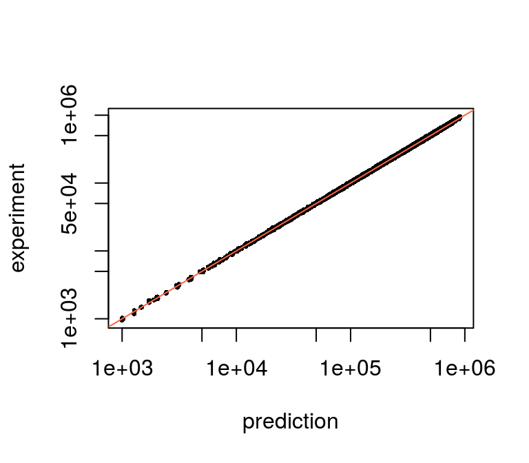
Model predictions vs. data
The data were simulated from known values in pulseRSpikeinsData$par and we can compare fit to the true values:
par(mfrow=c(1,2))
plot(par$d, fit$d, pch=16, cex=1,
     xlab="true", ylab="fit", main="d, degradation rate")
abline(0, 1, col = "tomato")
plot(par$mu, exp(fit$mu), pch=16, cex=1, log='xy',
     xlab="true", ylab="fit", main="mu, expression level")
abline(0, 1, col = "tomato")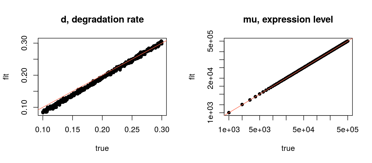
Fitted vs. true values
One can see, that there is a bias in the estimations: the normalisation affects the estimation by introducing a shift in the degradations rates. In this example, the normalisation and cross-contamination is derived on the basis of 5 labelled and 5 unlabelled spike-ins only.
For simulation the uniformly distributed parameters were used, which is also observed in the fitted values:
plot(exp(fit$mu), fit$d, pch=16, cex=.5, xlab="expression", ylab="degradation")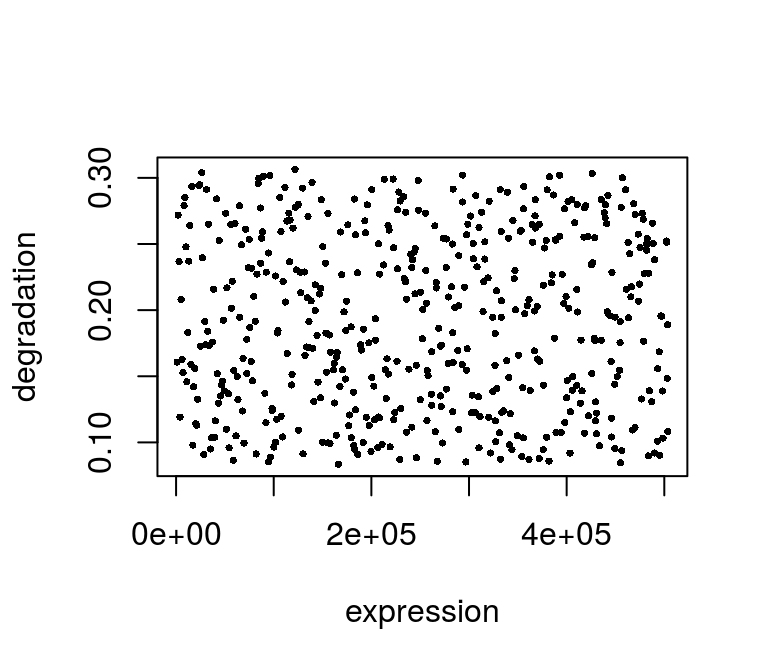
Parameter estimations
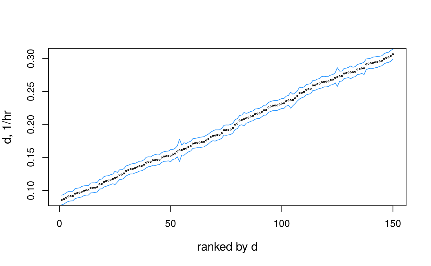
Confidence intervals
To generate the confidence intervals, one needs to provide the parameter name (e.g. “d”), indexes of the genes (in this example, only the first 150 genes), for which to compute the intervals and all the objects from the fitting procedure:
geneSubset <- 1:150
cis <- ciGene("d", geneSubset, pd, fit, opts)

## Create a result table and plot the CI together with the estimations
dat <- data.frame(
  d  = fit$d [geneSubset],
  mu = fit$mu[geneSubset],
  d.min = cis[,1],
  d.max = cis[,2]
)

o <- order(dat$d)
i <- seq_along(dat$d)
plot(x = i, y = dat$d[o], type = "n",
  cex.lab = 1.2,
  xlab = "ranked by d",
  ylab = "d, 1/hr"
)
lines(x = i, y = dat$d.max[o], col = "dodgerblue")
lines(x = i, y = dat$d.min[o], col = "dodgerblue")
points(x = i, y = dat$d[o], cex = .3)